Spin and Valley Physics in Two Dimensional Systems Graphene and Superconducting Transition Metal Dichalcogenides
Doctoral Thesis Defense
evansosenko.com/deck-doctoral-thesis
Background
2D Materials promise novel application
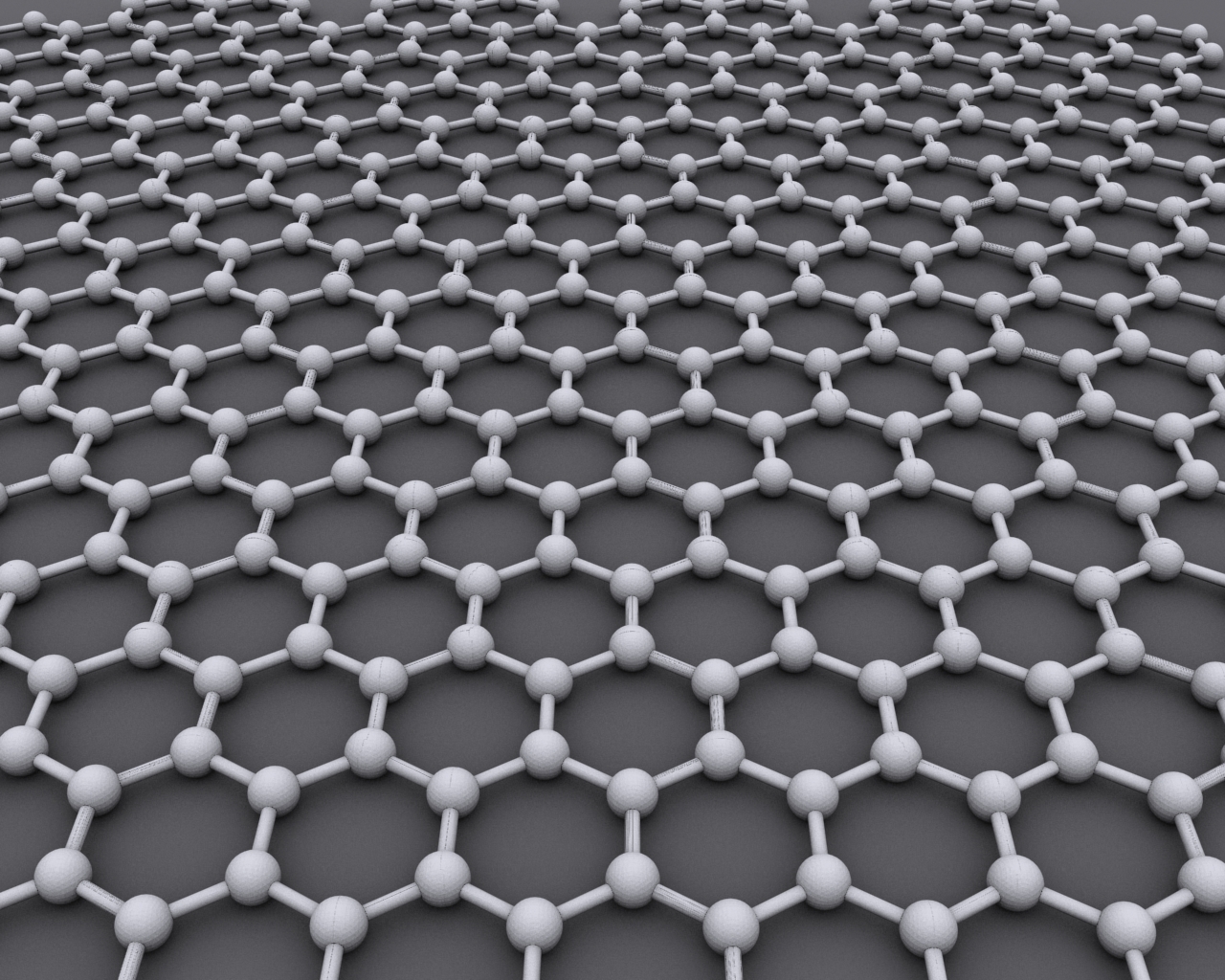
- Graphene discovered 2004
- 2D hexagonal carbon lattice, high electron mobility
- Relativistic low-energy model: Dirac cones, linear dispersion
- Strong, flexible & transparent
- Monolayer TMDs: also hexagonal lattice
- Gapped with strong spin-orbit coupling
- Both excellent candidates for spintronic devices
Spintronics
- Nobel Prize for GMR in 2007 (Albert Fert, Peter Grünberg)
- A future with devices built on spin-current
- Smaller and lower power
- Graphene? Predicted excellent conductor for spin-current
- TMDs? No spin degeneracy and spin couples to light polarization
Overview for Part I
Spin lifetime
- Injection, transmission, detection of spin signals
- Spin signals degrade via internal scattering
- Spin lifetime measures how quickly this happens
- Critical to find materials with long spin lifetimes
Motivation
- Theoretical predictions longer than measured: \( \text{ms} \) vs. \( \text{ps} \)
- Finite contact resistance mismatch: a potential candidate
- Unified analytic solution for fitting data in all limits

Outline
- Model and solution
- Hanle curve fitting
- Regimes and results
Device geometry
- \( L \) : contact spacing
- \( D \) : diffusion constant
- \( \tau \) : spin lifetime
- \( \lambda = \sqrt{D \tau} \)
- \( \omega = g \mu_B B / \hbar \)
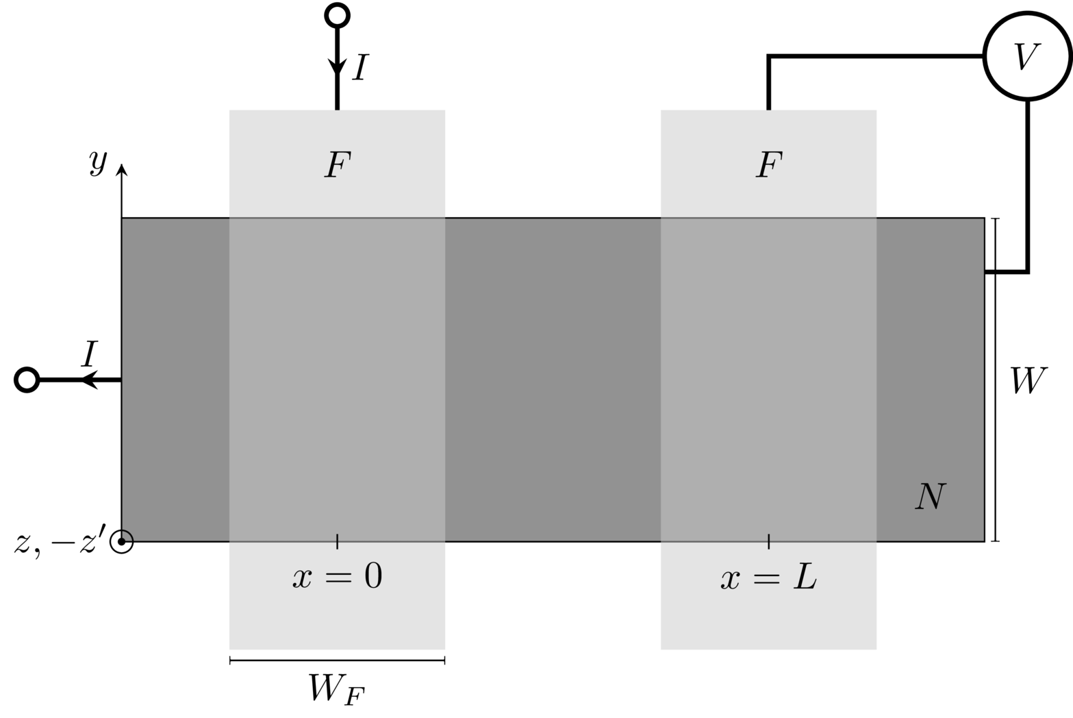
- \( \mu_s = \frac{1}{2} \left( \mu_{\uparrow} - \mu_{\downarrow} \right) \)
- \( J_{\uparrow \downarrow} = \sigma_{\uparrow \downarrow} \nabla \mu_{\uparrow \downarrow} \)
- \( J_{\uparrow \downarrow}^C = \Sigma_{\uparrow \downarrow} \left( \mu^N_{\uparrow \downarrow} - \mu^F_{\uparrow \downarrow} \right)_c \)
- \( J = J_{\uparrow} + J_{\downarrow} \)
- \( J_s = J_{\uparrow} - J_{\downarrow} \)
$$D \nabla^2 \mu_s - \frac{\mu_s}{\tau} + \omega \times \mu_s = 0$$
$$V \propto \mu_s^N(x = L)$$
$$R_\text{NL} = V / I$$
Fits
Tunneling contacts

- \( L = 2.1 \: \mu \text{m} \)
- \( P = 0.19 \: \)
- \( R_\text{C} = 2.03 \times 10^7 \: \text{k} \Omega \)
- \( \tau = 514.3 \: \text{ps} \)
- \( D = 0.02 \: \text{m}^2 \text{s}^{-1} \)
Tunneling contacts

- \( L = 5.5 \: \mu \text{m} \)
- \( P = 0.1 \: \)
- \( R_\text{C} = 6.70 \times 10^6 \: \text{k} \Omega \)
- \( \tau = 451.84 \: \text{ps} \)
- \( D = 0.01 \: \text{m}^2 \text{s}^{-1} \)
Fits
Pinhole contacts

- \( L = 3 \: \mu \text{m} \)
- \( P = 0.23 \: \)
- \( R_\text{C} = 2.31 \times 10^7 \: \text{k} \Omega \)
- \( \tau = 132.28 \: \text{ps} \)
- \( D = 0.02 \: \text{m}^2 \text{s}^{-1} \)
Transparent contacts

- \( L = 3 \: \mu \text{m} \)
- \( P = 0.01 \: \)
- \( R_\text{C} = 2.94 \: \text{k} \Omega \)
- \( \tau = 130.36 \: \text{ps} \)
- \( D = 0.04 \: \text{m}^2 \text{s}^{-1} \)
Fits: \( \tau \) Independent Limit
Transparent contacts

- \( L = 3 \: \mu \text{m} \)
- \( P = 0.02 \: \)
- \( R_\text{C} = 0.27 \: \text{k} \Omega \)
- \( \tau = 9.97 \times 10^9 \: \text{ps} \)
- \( D = 0.02 \: \text{m}^2 \text{s}^{-1} \)
Transparent contacts

- \( L = 3 \: \mu \text{m} \)
- \( P = 0.02 \: \)
- \( R_\text{C} = 0.28 \: \text{k} \Omega \)
- \( \tau = 9.95 \times 10^{13} \: \text{ps} \)
- \( D = 0.02 \: \text{m}^2 \text{s}^{-1} \)
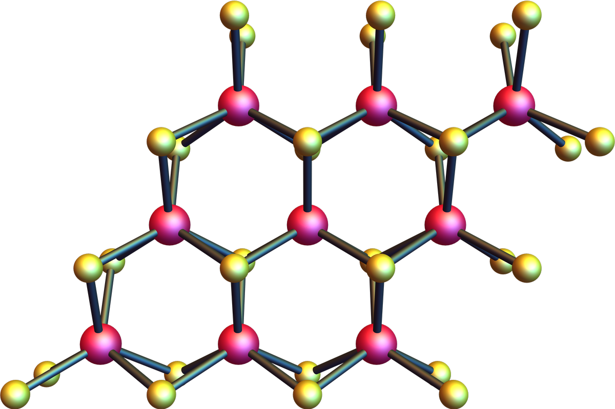
Transition metal dichalcogenides
- TMD overview and tight-biding, low-energy, two-valley model
- Optical valley selection rules and Berry curvature
- Intrinsic and induced superconductivity
- Intervalley and intravalley paring channels
- Superconducting optoelectronics and Berry curvature
TMD monolayers
- Direct band gap semiconductors: \( \mathrm{MoS_2} \), \( \mathrm{WS_2} \), \( \mathrm{MoSe_2} \), \( \mathrm{WSe_2} \)
- Break inversion symmetry ⇒ gapped out spectrum
- Two inequivalent valleys ⇒ new degree of freedom
- Strong spin-orbit coupling ⇒ large valance band spin-splitting
- Opposite valley Berry curvature
- Optical valley probe and valley Hall effect
- Two state tight binding model: \( d_{z^2} \), and \( d_{xy} \pm i d_{x^2 - y^2} \)

$$ H_{\tau}^0 \left( \mathbf{k} \right) = a t \left(\tau k_x \sigma_x + k_y \sigma_y \right) \otimes I_2 + \frac{\Delta}{2} \sigma_z \otimes I_2 - \lambda \tau \left(\sigma_z - 1 \right) \otimes S_z $$
D. Xiao, G.-B. Liu, W. Feng, X. Xu, and W. Yao, Phys. Rev. Lett. 108, 196802 (2012).Energy bands

- \( \Delta \)—band splitting
- \( \lambda \)—spin splitting
- \( \tau \)—valley index
- \( s \)—spin index
- \( a t = 3.15 \) Å eV
- \( \Delta = 1.66 \) eV
- \( 2 \lambda = 0.15 \) eV
- \( \mu = -0.83 \) eV
Optical excitations


Optoelectronic coupling
- Right circularly polarized light couples to right valley \( P_+ \)
- Left circularly polarized light couples to left valley \( P_- \)
Valley Hall effect

Semiclassical equations
\( \dot{\mathbf{r}} = \nabla_{\mathbf{k}} E \left( \mathbf{k} \right) - \dot{\mathbf{k}} \times \mathbf{\Omega} \left( \mathbf{k} \right) \)
\( \dot{\mathbf{k}} = -e \mathbf{E} - e \dot{\mathbf{r}} \times \mathbf{B} \)
Anomalous velocity
\( \mathbf{v} = e \mathbf{\Omega} \left( \mathbf{k} \right) \times \mathbf{E} \)
Berry curvature
\( \mathbf{\Omega}_{\tau \sigma}^n \left( \mathbf{k} \right) = \nabla_{\mathbf{k}} \times \left\langle u_{\tau \sigma}^n \left( \mathbf{k} \right) \right\rvert i \nabla_{\mathbf{k}} \left\lvert u_{\tau \sigma}^n \left( \mathbf{k} \right) \right\rangle \)
Broken inversion symmetry
\( \mathbf{\Omega}_{\tau, \sigma}^n \left( \mathbf{k} \right) = - \mathbf{\Omega}_{-\tau, \sigma}^n \left( \mathbf{k} \right) \neq 0 \)
Superconducting channels
Induced
$$ \Delta_{\mathbf{k}} = \frac{1}{2} \left( B_+ + B_- \right) - \frac{1}{2} \left( B_+ - B_- \right) \cos{\theta_{\mathbf{k}}} $$
Intrinsic
$$ \Delta_{\mathbf{k}} = \chi_0 \cdot f_{\mathbf{k}} $$
Gap equation
$$ \chi_0 = \frac{v_0}{2} \sum_{\mathbf{k}} \frac{f_{\mathbf{k}} \cdot \chi_0}{\lambda_{\mathbf{k}}} \bar{f}_{\mathbf{k}} $$

- Project into upper-valance bands (\( \tau = s \))
- Mean field theory BCS-type solutions: gap function \( \Delta_{\mathbf{k}} \)
- Different \( f_{\mathbf{k}} \) per channel
- \( m = 0 \) intervalley channel always dominates
- Both classes give constant gap function for dominant paring
Optical coupling

- \( \mathbf{A} / A_0 = \mathbf{\epsilon} e^{i \omega t} + \mathbf{\epsilon}^* e^{-i \omega t} \), \( \mathbf{k} \rightarrow \mathbf{k} + e \mathbf{A} \)
- Harmonic perturbation ⇒ correlated phase's optical transition rates
- Valley selection remains coupled to circularly polarized light
Berry curvature

- BCS ground state has zero net curvature
- Optical pair-breaking ⇒ selectively excite carriers in single valley
- Berry curvature retains relative sign relations